QUESTION 1

Background

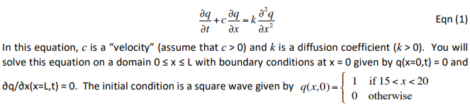
In this question we consider the 1-D advection-diffusion equation:

Q1a By hand, write the forward in time, centred in space (FTCS) difference equation that approximates equation (3). What is the temporal and spatial order of accuracy of this discretization?

Q1b Undertake a von Nuemann stability analysis for this difference equation (you can assume that the error satisfies the same difference equation as the solution for q, because it does). Consider just ONE Fourier mode of the representation of the error, and write it in the simplified form

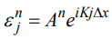
Write an expression for the amplification factor (i.e. the ratio of error at time n+1 to that at time n) and replace any complex exponential terms by expressions involving sin and cos - it will be a complex number. Simplify as far as you can, but you do NOT need to derive the stability criterion.

Q1c Undertake a Taylor series stability analysis - i.e. expand each term in the finite difference equation about time n, location j, as done in workshops and replace the time derivative operator with a spatial derivative operator that looks like

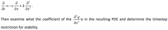
Q1d Write a MATLAB function that updates the values of q by ONE TIMESTEP using the FTCS scheme (it will be a short function). Ensure that your function has the function header

function [q_new] = ftcs_step(q,dt,dx,c,k)

The boundary condition at x=0 is easily implemented using q(x=0)=0, but you will need to set the boundary condition at x=L using a finite difference approximation to the derivative. Thus, when q(L,t) is needed in an expression, you will need to use the finite difference expression of the derivative to set the BC. (In this lab, centered or one-sided differences are OK to use for the BC - whatever you like).

Q1e

Modify the template in Lab06_Q1.m using the following values

• Set L = 100

• Discretise your domain with 250 intervals.

• Choose c = 1.0

• Set tmax = 60

Choose 3 values of k [0.01, 0.1, 1.0] and integrate forward in time until t = tmax with the following CFL1 numbers: [0.01, 0.1, 0.25] and (i.e. you will have 9 solutions).

Create a single plot with 9 subplots. Each subplot will have the solution for one CFL number and one value of k. In each subplot, plot the solution at approximately every 20 time units (i.e. at t = 0, 20, 40, 60) on the same subplot (i.e. you should have 9 subplots, each with 4 curves). The plot times can be “approximate” (e.g. 19.95 is close enough to 20). ALSO include a plot of the analytic solution of the advection-only problem at each time in a different colour in each subplot for comparison (giving 8 curves per subplot).

Describe the key features of what you are seeing as you change k and the CFL number and suggest WHY you observe what you observe (the following hints might help you)

HINTS:

1) The FTCS scheme for equation 3 when k=0 (i.e. pure advection) is unconditionally unstable.

2) The FTCS scheme for equation 3 when c = 0 (i.e. pure diffusion) is conditionally stable. The condition for stability is discussed in the lecture notes.

3) The answer to Q1c could provide some insight.

data.all.m