On Moodle, you have been given a data set that is saved as a CSV file. The data set contains the signal intensity f(t) of a fluorescent drug as it diffuses into a live cell as a function of time 0 ≤t ≤ 10 s. The cellular diffusion commences at t = 2 seconds and the data from 0 ≤ t< 2 sis noise. Your overall goal here is to write a Python program that imports this data and calculates the derivative of the signal at t = 3 seconds. We'll tackle this step by step:

a) Import the dataset in Python and approximate the signal derivative using the forward difference approximation. Have your program output a figure window called Raw Signal and Raw Derivative that contains two subplots (a 1x2 matrix of plots - use the subplot command). The subplot on the left is a plot of f(t) versus time from 0 ≤ t ≤ 10 s, use black dots to represent the data. The subplot on the right is the derivative df(t)/dt of the signal as a function of time - use blue dots to represent this function. Label your axes.

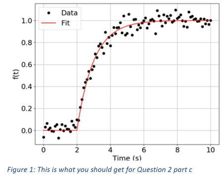
b) A common problem with numerical derivatives applied to noisy data. Almost always, we'll need a way to pre-process the data before we can take a numerical derivative. This is because the difference algorithms are very sensitive to noise. If we know or can reasonably hypothesize as to the form of the underlying function of the data, one such way to clean up the data' before taking our numerical derivative is to fit this data. Using a nonlinear least squares method, fit the data f(t) over 2 ≤ t ≤ 10 s to the following equation: Yfit(t) = 1 – exp(a(t – 2)) where a is a free parameter. Set the initial guess for a to be within – 1.1 ≤ a ≤ -0.9. The form of this equation was based on the fact that we'd expect an exponential-like curve for this type of diffusion problem and that the drug uptake starts at t = 2. Have your program output a second figure window called Raw Signal and Fitted Signal. On this figure, plot the raw data using black dots and overlay the fit using a red line. Label your axes and add a legend. Note here that we don't want to fit the noise floor data from 0 ≤ t< 2 s since these residuals will ultimately go into our nonlinear least squares calculations. The data of interest here is from t ≥ 2 s, and so once you have fit this data, you can set the model fit to 0 from 0 ≤ t < 2. Your figure for this question should look like that depicted below.

c) Now that we have a best-fit formula for this raw data yfit(t), we can now take the numerical derivative of this function dyfit/dt. We can take this derivative numerically or analytically. If you take this derivative numerically, use the forward difference method. Output a third figure window called Fitted Signal and Derivative from Fit. On this plot, plot the fitted signal in red, and overlay the derivative of this fit in blue dots. Finally, output using a print statement the value of the derivative of this fit at t = 3s.

Data