Task 4

In this task, you will be able to apply differential equations to engineering problems.

Scenario: It is widely use differential equations with boundary condition to model the electrical systems. In this task, analytical and numerical methods to solve the solution of differential equation with initial boundary condition need to be applied.

Task 4.1 (P4.1)

In an alternating current circuit containing resistance R and inductance L the current i is given by:

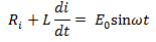
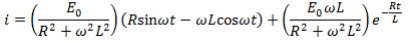
Given i = 0 when t = 0, select appropriate differential equation model to show that the solution of the equation is given by: (hint: partial differential model to set up second order differential equation or others).

Task 4.2 (P4.2)

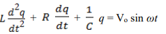
represents the variation of capacitor charge in an electric circuit.

Given that R = 40 omega , L = 0.02H, C = 50 10-6 F, V0 = 540.8V and omega = 200 rad/s and also

given the boundary conditions that when t = 0, q =0 and dq/dt = 4.8.

Solve problem using initial and boundary value conditions to determine an expression for q at t second.

Task 4.3 (P4.3)

Obtain a numerical solution of the differential equation

dy/dx = 3(1+x)-y

Given the initial conditions that x=1 when y=4 for the range x=2.0 with intervals of 0.2.

Solve differential equations numerically using mathematical software.

ii) Find the value of y if x = 1.58, dy/dx = 0.5