In the Labs

Design, create, modify, and/or use a workbook following the guidelines, concepts, and skills presented in this module. Labs 1 and 2, which increase in difficulty, require you to create solutions based on what you learned in the module; Lab 3 requires you to apply your creative thinking and problem-solving skills to design and implement a solution.

Lab 1: Using a Master Sheet to Create a Multiple-Sheet Workbook

Note: To complete this assignment, you will be required to use the Data Files. Please contact your instructor for information about accessing the Data Files.

Problem:

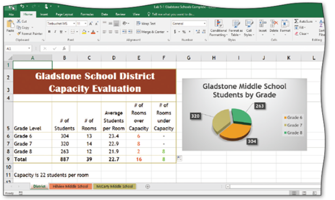
You are part of a task force assessing the classroom capacities of the middle schools in your district. You have been charged with creating a master worksheet for the district and separate worksheets for each of the two middle schools. The middle school worksheets should be based on the district worksheet. Once the worksheets have been created, the middle school data can be entered into the appropriate worksheets, and the district worksheet will reflect district-wide information. The district worksheet appears as shown in Figure 5–74.

Figure 5–74

Perform the following tasks:

1. Run Excel. Open the workbook Lab 5 – 1 Gladstone Schools from the Data Files. Save the workbook using the file name Lab 5 – 1Gladstone Schools Complete.

2. Add two worksheets to the workbook after Sheet1 and then paste the contents of Sheet1 to the two empty worksheets.

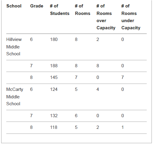
3. From left to right, rename the sheet tabs District, Hillview Middle School, and McCarty Middle School. Color the tabs as shown in Figure 5–74 . On each of the school worksheets, change the title in cellB2 to match the sheet tab name. On each worksheet, fill the rangeA2:F3 to match the color of its sheet tab. Enter the data in Table 5–8 into the school worksheets.

Table 5–8

Middle School Classroom Capacity Figures

4. On the two school worksheets, calculate Average Students per Room in column D and totals in row 9.

5. On the District worksheet, use the SUM function, 3-D references, and copy-and-paste capabilities of Excel to populate the ranges B6:C8 andE6:F8. First, compute the sum in cells B6:C6 and E6:F6, and then copy the ranges B6:D6 and E6:F6 through ranges B7:C8 and E7:F8respectively. Finally, calculate average students per room for the district for each grade level, and for the district as a whole.

6. Select the range E6:E9 on the District worksheet. Select all the worksheets and then use the Format Cells dialog box to apply a custom format of [Red]#,###;;“-”.

7. Select the range F6:F9 on the District worksheet. Select all the worksheets and then use the Format Cells dialog box to apply a custom format that will format all nonzero numbers similar to the format applied in Step 6 but with green for nonzero entries.

8. Use the Cell Styles button (Home tab | Styles group) to create a new cell style named My Title. Use the Format button (Styles dialog box) to create a format. Use the Font sheet (Format Cells dialog box) to select the Britannic Bold font, a font size of 22, and a white font color. Check only the Alignment and Font check boxes in the Style dialog box.

9. Select cells A2:A3 on the District worksheet. Select all the worksheets. Apply the My Title style to the cell.

10. Using Figure 5–74 as a guide, add borders to the worksheets. The borders should be the same on all worksheets.

11. Select the District worksheet. Create a 3-D pie chart using the rangeA6:B8. Edit the title to match Figure 5–74. Apply the Chart Style 3 to the chart.

12. Move the chart to the right of the data. Right-click the pie to display the shortcut menu and then click ‘Format Data Series’ to open the Format Data Series task pane. Set the Pie Explosion to 10% to off set all of the slices.

13. Select the chart area and display the Format Chart Area task pane. Set the X rotation to 100°.

14. Use the Chart Elements button to display the Data Labels submenu. Click More Options. Select only the Value and ‘Show Leader Lines’ options. Choose the Outside End label position and adjust the labels as necessary to display the leader lines.

15. If requested by your instructor, enter the text Prepared by followed by your name in the header, on the left side.

16. Save the workbook. Submit the revised workbook as specified by your instructor.

17. Did you calculate an average in cell D9 using the data in column D or the data in row 9? Explain the reasoning for your choice.

Lab 2:

Note: To complete this assignment, you will be required to use the Data Files. Please contact your instructor for information about accessing the Data Files.

Problem:

The Apply Your Knowledge exercise in this module calls for consolidating the payroll data from four worksheets to a fifth worksheet in the same workbook. This exercise takes the same data, this time stored in four separate workbooks, and then consolidates the total sales and total commission by linking to a fifth workbook.

Part 1: Perform the following tasks:

1. If necessary, copy the following five files from the Data Files to the location at which you save your solution files. Lab 5 – 2 Commission Annual, Lab 5 – 2 Commission Quarter 1, Lab 5 – 2 Commission Quarter 2, Lab 5 – 2 Commission Quarter 3, and Lab 5 – 2Commission Quarter 4. Run Excel. Using the Search box with the term, commission, open the five files.

2. Use the Switch Windows button (View tab | Window group) to make Lab 5 – 2 Commission Annual the active workbook. Save the workbook in the same location, using the file name, Lab 5 – 2Commission Annual Complete.

3. Select cell C9. Click the Sum button (Home tab | Editing group) and then switch to the Lab 5 – 2 Commission Quarter 1 workbook. When the workbook is displayed, click cell D9, change the absolute cell reference $D$9 in the formula bar to the relative cell reference by deleting the dollar signs. Click immediately after D9 in the formula bar and then press the comma key.

4. Switch to the Lab 5 – 2 Commission Quarter 2 workbook. When the workbook is displayed, click cell D9, change the absolute cell reference $D$9 to D9, click immediately after D9 in the formula bar, and then press the comma key.

5. Repeat Step 3 for the Quarter 3 and Quarter 4 workbooks. After adding the Quarter 4 workbook reference, press the enter key rather than the comma key to sum the four quarter sales figures. The annual total sales for employee DK52 should be $221,500.00 as shown in Figure 5–75.

6. With the workbook Lab 5 – 2 Commission Annual Complete window active, select cell C9 and drag the fill handle through D9 to display total commission for employee DK52.

7. Select cells D9 and C9. Drag the fill handle through cell D13 to display the total sales and total commission for all employees, and as annual totals. When the Auto Fill Options button is displayed next to cell D14,click the Auto Fill Options button and then click ‘Fill Without Formatting’.

8. Save and close all workbooks. Submit the solution as specified by your instructor.

Dataset