Indy Car
You have been hired to analyze the effectiveness of carbon hardening additives to Indy car tires. The added carbon increases the puncture strength and you will analyze its impact on burn temperature and weight. You will use Excel's statistical functions and the Analysis ToolPak to complete the next steps. Refer to Figure 8.29 as you complete this exercise.
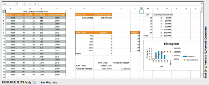
a. Open e08p2IndyCar and save it as e08p2IndyCar_LastFirst.
b. Click cell H4 in the Tires worksheet. Type =CORREL and press Tab. Select the range C4:C23 for the first argument, press comma, and then select the range E4:E23 for the second argument. Press CTRL+Enter.
c. Click cell 14. Type =STDEV.S and press Tab. Select the range E4:E23 and press Ctrl+Enter.
d. Select the range 110:116. Type =FREQUENCY and press Tab. Select the range E4:E23 and press comma. Select the range H10:H15 and press Ctrl+Shift+Enter.
e. Load the Analysis ToolPak by completing the following steps, or if it is already available, skip to Step f.
• Click the File tab.
• Click Options and select Add-ins on the left side of the Excel Options dialog box.
• Select Excel Add-ins in the Manage box and click Go.
• Click Analysis ToolPak in the Add-ins window and click OK.
f. Click the Data tab and click Data Analysis in the Analysis group. Select Histogram, click OK, and then complete the following steps:
• Type D4:D23 in the Input Range box.
• Type K10:K15 in the Bin Range box.
• Type M3 in the Output Range box.
• Click the Cumulative Percentage option.
• Click chart.
• Click OK.
• Position the chart so the upper-left corner starts in cell M12 and resize it so the chart fills the range M12:R20.
g. Click the Data tab and click Data Analysis in the Analysis group. Select Covariance, click OK, and then complete the following steps:
• Type E3:F23 in the Input Range box.
• Click Columns.
• Click Labels in first row.
• Type H19 in the Output Range box.
• Click OK
• Resize columns H:J and M:0 as needed.
h. Click the Test Drive worksheet. Click the Data tab and click Data Analysis in the Analysis group. Select ANOVA: Single Factor, click OK, and then complete the following steps:
• Type C2:E21 in the Input Range box.
• Click Columns.
• Click Labels in first row.
• Type G2 in the Output Range box.
• Click OK
• Resize Columns G:M as needed.
i. Select the range B2:C21, click Data tab, click Forecast Sheet, and click Create.
j. Rename the newly created worksheet Forecast and resize the chart as needed.
k. Create a footer on all worksheets with your name on the left side, the sheet name code in the center, and the file name code on the right side.
l. Save and close the workbook. Based on your instructor's directions, submit e08p2IndyCar_LastFirst.


 Login | Sign Up

