a. Open e03p1Utilities and save it as e03p1Utilities_LastFirst.
b. Select the range A4:E17. click Quick Analysis, click Charts, and then click Clustered Column.
c. Click Chart Filters to the right of the chart and do the following:
• Deselect the Monthly Totals check box in the Series group.
• Scroll through the Categories group and deselect the Yearly Totals check box.
• Click Apply to remove totals from the chart. Click Chart Filters to close the menu.
d. Point to the chart area. When you see the Chart Area Screen Tip, drag the chart so that the top-left corner of the chart is in cell A21.
e. Click the Format tab and change the size by doing the following:
• Click in the Shape Width box in the Size group, type 6", and then press Enter.
• Click in the Shape Height box in the Size group, type 3.5", and then press Enter.
f. Click the Design tab, click Quick Layout in the Chart Layouts group, and then click Layout 3.
g. Select the Chart Title placeholder, type Monthly Utility Expenses for 2018, and then press Enter.
h. Click the chart, click the More button in the Chart Styles group, and then click Style 6.
i. Click Copy on the Home tab, click cell A39, and then click Paste. With the second chart selected, do the following:
• Click the Design tab, click Change Chart Type in the Type group, click Line on the left side of the dialog box, select Line with Markers in the top-center section, and then click OK.
• Click the Electric data series line to select it and click the highest marker to select only that marker. Click Chart Elements and click Data Labels.
• Repeat and adapt the previous bulleted step to add a data label to the highest markers for Gas and Water. Click Chart Elements to close the menu.
• Select the chart, copy it, and then paste it in cell A57.
j. Ensure that the third chart is selected and do the following:
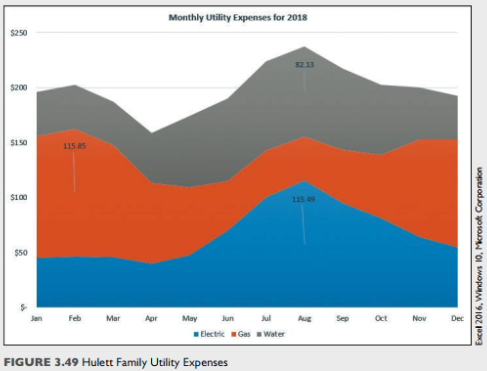
• Click the Design tab, click Change Chart Type in the Type group, select Area on the left side, click Stacked Area, and then click OK.
• Click Move Chart in the Location group, click New sheet, type Area Chart, and then click OK
• Select each data label and change the font size to 12. Move each data label up closer to the top of the respective shaded area.
• Select the value axis and change the font size to 12.
• Right-click the value axis and select Format Axis. Scroll down in the Format Axis task pane, click Number, click in the Decimal places box, and then type 0. Close the format Axis task pane.
• Change the font size to 12 for the category axis and the legend.
k. Click the Expenses sheet tab, select the line chart, and do the following:
• Click the Design tab, click Move Chart in the Location group, click New sheet, type Line Chart, and then click OK.
• Change the font size to 12 for the value axis, category axis, data labels, and legend.
• Format the vertical axis with zero decimal places.
• Right-click the chart area, select Format Chart Area, click Fill, click Gradient fill click the Preset gradients arrow, and then select Light Gradient - Accent 1. Close the
Format Chart Area task pane.
l. Click the Expenses sheet, select the range B5:016 and do the following:
• Click the Insert tab, click Line in the Sparkline group, click in the Location Range box, type B18:D18, and then click OK.
• Click the High Point check box to select it and click the Low Point check box to select it in the Show group with all three sparklines selected.
m. Create a footer with your name on the left side, the sheet name code in the center, and the file name code on the right of each sheet.
n. Save and close the file. Based on your instructor's directions, submit eo3pl_Utilities_Last First.


 Login | Sign Up

