Part A: Hodgkin-Huxley model

*** Remember to include: 1. your code (as an appendix) and 2. a statement of collaboration. ***

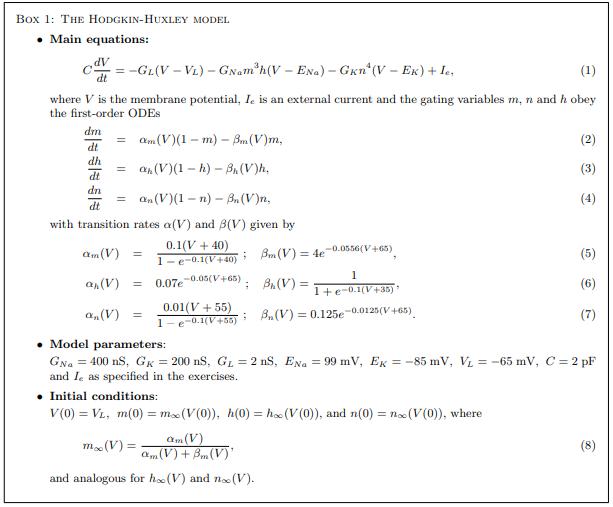
1. (Main simulation) Simulate tmax = 200 ms evolution of one HH neuron as defined in Box 1. Use the forward Euler algorithm with time step dt = 0.01 ms. Stimulate the neuron from time t0 = 40 ms with a constant current of amplitude I0 = 200 pA and lasting until tmax (i.e., Ie = 0 for t < 40 ms and Ie = I0 for t > 40 ms). Plot in the same figure but in different subplots:

i) the membrane potential vs. time,

ii) the total membrane current, Im = GL(V − VL) + GNam3h(V − ENa) + GKn 4 (V − EK), vs. time,

iii) the sodium conductance (=GNam3h) vs. time,

iv) the potassium conductance (=GKn 4 ) vs. time, and v) the current Ie vs. time.

Include the plot in your report.

Matlab tip ⇒ Use figure(1) and then start each plot with subplot(5,1,x), where x ranges from 1 to 5.

2. (Spike detection) Endow your code with a mechanism to detect each ‘spike’ (=action potential). To do so, you must decide on a critical value Vspk at which you might say that a spike has been emitted (values between −30 and 0 mV should be good choices). Make sure to count each spike only once. Now, enlarge the previous plot from Exercise 1 to illustrate the dynamics of one single action potential, marking the time at which Vspk was reached. Include the plot in your report.

Matlab tip ⇒ Use xlim([t1 t2]) in each subplot to zoom in all subplots equally; choose as t1 and t2 the time just before and just after the action potential, respectively

3. (Action potential threshold) Determine the threshold current to elicit a single action potential. Start from a very small value of the input current (e.g., I0 = 2 pA) and increase it until you find the value of the current I1 at which the neuron starts firing one action potential only, and then stops firing. Report the value I1 in your report.

4. (Rheobase current) By increasing the current beyond the value I1, eventually 2, 3 or more action potentials will be generated, but then the neuron stops firing again. By increasing the current even more, eventually repetitive firing ignites (i.e., the neuron doesn’t stop firing). Find Irh, defined as the smallest value of the current above which repetitive firing ignites. Report the value Irh in your report.

5. (f − I curve) The previous exercise seems to imply that the HH model will switch from having zero firing rate to having a finite firing rate at a critical value Irh. Run Exercise 1 again, this time for at least 40 values of the current with increasing amplitude, starting from values a bit lower than I = Irh. For each run, estimate the firing rate in that run, and then plot the current-frequency response function once all firing rates have been estimated (see Box 2 below for the relevant definitions).

Important: Assign zero firing rate in the case of no spikes; and assign zero firing rate every time the neuron emits a few action potentials and then stops firing. In all other cases (repetitive firing) the firing rate will be a positive number. When plotting the firing rate vs. the amplitude of the input current, make sure to include the simulations which resulted in zero firing rates.

Include the plot of the f-I curve in your report and answer the following questions:

i) Describe briefly the salient characteristics of this f − I curve.

ii) Via the f − I curve, can you get an independent estimate of Irh? Can you locate Irh on the plot?

iii) Imagine you wanted to use this model neuron to encode a graded input (i.e., spanning a continuous range of input currents) into the neuron’s output firing rate. Does this f − I curve suggest that this would be an efficient way to do so? Why or why not?

Box 2: Firing rate estimation

The Current-frequency response function (or ‘f − I curve’ for short) is the curve depicting the firing rate as a function of the amplitude of the input current Ie.

You can calculate the firing rate in either of two ways:

i) as the number of spikes per second between t0 and tmax (make sure to use a longer simulation time tmax, e.g., 2000 ms, to obtain better estimates of the firing rates);

ii) as the inverse of the mean inter-spike interval (ISI), where the ISI is the interval of time between two successive action potentials.

Use method ii) as it is more accurate (if you try out both methods you will be able to notice the difference. Can you tell what is the reason behind this difference?). Note that either method requires the use of the spike detection mechanism developed in Exercise 2 (make sure to count each spike only once!).