Scenario

Your supervisor has been assigned to be the interim deputy assistant national operations manager of the Liberty Credit Union organization, a credit union with over 350 branches nationwide. The role directly serves the office of the Chief Operations Officer, which oversees national marketing and operations for the organization. The previous manager left suddenly and retired after serving in that role for 10 years, during which time the organization weathered many economic storms and regulatory changes. The Chief Operations Officer has scheduled an offsite planning meeting to discuss a new strategy for the direction of the Liberty Credit Union. Your supervisor will be providing a report about a proposed strategy for growth in sales based on analysis of products and regional performance, and he has asked you to prepare a workbook to support his presentation at the upcoming meeting.

You plan to analyze the data using standard statistical methods in Microsoft Excel and develop statistics as well as charts and graphs to support the presentation of data. Your task is to conduct data analysis and prepare a final report for your supervisor about your findings, which will also include an analysis of the data and how it informs a future strategy for growth.

Once you have reviewed the scenario, review the project overview, approximate time commitment, and competencies that you will be responsible for in this project.

Step 1: Refresh Your Math, Statistics, and Excel Skills

Step 2: Opening and Saving an Excel Spreadsheet

Click to reveal instructions for TLP students

1. Download the TLP data set TLP data set template and take a few minutes to review the Help Desk dataset. Note: There are two worksheets or tabs. The first tab (titled "QR Analysis Essay") will be where you cut and paste your end-of-project essay. We'll work through these problems in the next steps.  The second tab (titled "Data ") contains the data to be analyzed.

2. Open the Excel file and go to Save As to rename it. Use the name format YourLastName Project 4. This file contains the data that you will manipulate and analyze. You will add tabs in the next steps to build an Excel workbook for this project.

3. Properly format Excel workbook. Set the margins for landscape with narrow margins. Enter your name, date, and page number in the footer area of the sheet. Format the entire spreadsheet using Calibri 11-point font.

Now that you have completed these tasks, proceed to the next step.

Step 3: Add Data

Click to reveal instructions for TLP students

In Section 1 on the Data tab, complete each blank column of the spreadsheet to arrive at the desired calculations. Use Excel formulas to demonstrate that you can perform the calculations. Remember, a cell address is the combination of a column and a row. For example, C11 refers to Column C, Row 11 in a spreadsheet.

Reminder: Occasionally in Excel, you will create an unintentional circular reference. This means that within a formula in a cell, you directly or indirectly referred back to the cell. For example, while entering a formula in A3, you enter =A1+A2+A3. This is not correct and will result in an error. Excel allows you to remove or allow these references.

Hint: Another helpful feature in Excel is Paste Special. Mastering this feature allows you to copy and paste all elements of a cell, or just select elements like the formula, the value, or the formatting.

Ready to Begin?

1. To calculate assets per member, you will divide the total assets by the member count using cell referencing. In cell E11, enter =D11/H11, which will calculate the assets per member by dividing D11, total assets for the first listed credit union, by H11, which contains the member count for that credit union. Once you have the answer displayed, you will then copy this formula down the column. Click the cell with the formula to be copied, move your cursor to the bottom right of the cell until it becomes a plus sign, then click and drag to the bottom of the table. This will copy the formula and Excel will increment the references so that you only need to type the formula once.

2. In Column F, calculate the number of years each credit union has been open by creating a formula that incorporates the date in cell F9 and demonstrates your understanding of relative and absolute cells in Excel. You will need a formula that can compute absolute values to determine years of service. You could do this longhand, but it would take you a long time. So, try the YEARFRAC formula, which computes the number of years (and even rounds for you). Once you start the formula in Excel, the element will appear to guide you. You need to know the ending date (F9) and the opening date (B11). The formula looks like this: =YEARFRAC($F$9,B11), and the $ will repeat the formula calculation down the column if you grab the edge of the cell and drag it to the bottom of the column, as above.

3. To determine if a credit union is mature, use an IF statement in Column I to flag with a "Yes" any credit union in business for 10 years or more. Here is how an IF statement works: =IF(X is greater (or less than) Y, “Answer”, IF not, “Answer”). Expressed as a formula, the IF statement would look like this: =IF(F11>=10,"Yes","No"). You can drag this formula down the column or highlight the starting cell, hold down the shift key, scroll down to cell 382, and release, and the whole column should compute properly.

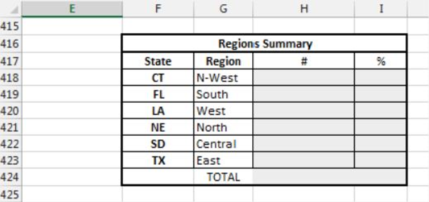
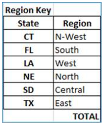
4. Using the VLOOKUP function, use the Region Key located at F417:G423 to fill in the cells in Column N to identify the region in which the employee is located based on the state listed in Column M. (If this function is new to you, hang in there—this one is worth it.)

There are some video resources available, one listed below, that address common challenges in this Excel assignment. Do not be confused if you see a data set that is different from yours—the principles are the same! Remember, if you have any questions, ask.

Source: Used with permission from Microsoft.

You will devise a formula that will match the state to a region (in position 2). We will use the $ function to enable a repeat of the formula down the column. =VLOOKUP(M11,$F$417:$G$423,2,FALSE)

To view videos that explain these formulas, please refer back to Step 1 under the link entitled Access Tutoring Help and Other Resources. The videos were created for another class but pertain to this same data set.

Step 4: Use Functions to Summarize the Data

In this step, you'll begin to see patterns in the data that inform the “story” of the data table that you have prepared up to this point.

Click to reveal instructions for TLP students

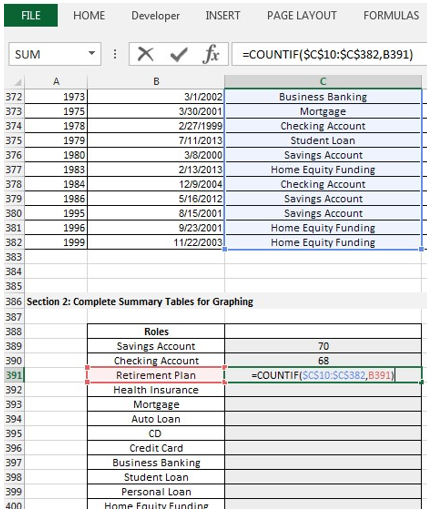
You are now ready to move into Section 2 and prepare the data for future analysis. You will include some simple statistical analyses as well as charts and graphs to present the data. Start by presenting the categories of data in summary tables, then counting them, totaling them, and calculating percentages. This basic analysis helps you begin to describe patterns in the data and starts to form the “story” of the workforce.

Complete each table in Section 2. Use the  countif function to count each item in each table. Use the  sum function to total the tables when required. Calculate percentages for each table as required. Format cells appropriately. Remember to make smart use of reference cells in formulas (avoid typing in numbers or text into formulas—instead point to other cells) and use mixed and fixed cell references to make copying formulas faster and easier. Your supervisor will look for your appropriate use of these tools!

Source: Used with permission from Microsoft.

Now, you are going to project sales for 2017–2020 by using the forecast tool in the Data tab.

Source: Used with permission from Microsoft.

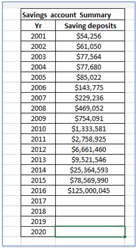
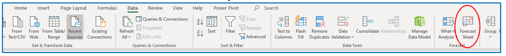
To use the Forecast tool to apply a formula to existing sales, highlight the savings amounts for 2001–2016 and select the Forecast tool on your Datatab.

Source: Used with permission from Microsoft.

You will get a quick forecast with low, median, and high projections for the years. If you choose "Create" on that sheet, you will get a more nuanced complete analysis for the years 2017–2020. Fill in those numbers in Savings Count Summary in Section II.

With this step complete, proceed to the next step, where you will begin your analysis.

Step 5: Add Information to Your Spreadsheet

In this step, things get interesting! You will expand your analysis by employing descriptive statistics, or summary statistics, using Excel formulas. Now you will calculate mean, median, and mode for the categories of data and derive the deviation, variance, dispersion, and distribution. Format all the results to two decimal places.

In Section 3 of the data sheet, use the appropriate Excel function to complete the table, calculating summary statistics of Total Assets, Assets per Member, Years of Service, Directors, and Member Count. Use the summary statistic Excel functions of =AVERAGE, =MEDIAN, = MODE, = STDEV.S, =VAR.S, =KURT, = SKEW, = MIN, =MAX, =SUM, and =COUNT to derive these statistics for the three data categories. Standard error and range should also be calculated.

Your data set in Tab 1: DATA should be built when you have completed this step.

Step 6: Use the Data Analysis Toolpak

Now that you have calculated descriptive statistics using individual Excel functions, we'll look at another approach. Did you know that you can generate the same descriptive statistics in one easy step?

Now, you will use Excel's built-in Analysis Toolpak, an add-in that allows you to work with statistics and confirm the answers of your summary statistics. It will help you to save time by performing various complex analyses based on your needs.

You will first need to make sure the toolpak is enabled. Feel free to references How to Enable Data Analysis Toolpak for assistance. When you have completed that process successfully, you will see the words "Data Analysis" or an icon on the top right corner on the Data tab. Select Data Analysis and then choose Descriptive Analysis from the list.

Note: There may be some minor differences in the answers depending on the version of Excel you are using. Mac users will need Excel 2016 or later to download the toolpak.

Then proceed to the instructions that match your current program to calculate the statistics using the toolpak:

Click to reveal instructions for Tranformational Leadership Program students.

A. Calculate the statistics. You can perform these calculations in one step by highlighting the adjacent columns of data in D10:H382. Place the output on a new sheet in the workbook. Label the tab "Excel Summary Stats."

B. Compare your calculations from the data analysis feature to the results you got in the previous step, using individual functions.

Step 7: Create Visual Representations of the Data: Charts and Graphs 

Where would we be without the ability to view data in charts? It is sometimes easier to grasp the context of data if we can see it captured in an image. Graphs and charts help readers digest and interpret information more quickly, consistent with the familiar adage "a picture is worth a thousand words."

Working with Excel Charts will provide an overview of the type of charts available such as pie and bar charts. Refer to it to create a histogram along with Use the Analysis Toolpak as needed. 

Click to reveal instructions for Transformational Leadership Program (TLP) students.

Create the following graphs in your workbook on a separate tab named "Graphs & Charts":

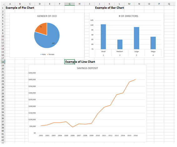
A. Create separate pie charts that show the percentage breakdown by (a) gender, (b) number of data analyst on staff, and (c) marital status. Explore pie chart formats.

B. Create separate bar charts that show the (a) number of directors, and (b) number of credit unions per state.

C. Create a line graph for the savings account deposits.

Source: Used with permission from Microsoft.

D. Create a histogram that shows the assets per member in incremental assets of $5,000. Show how many credit unions have assets per member in the following ranges: < $1,000; $1,000–$6,000; $6,000–$11,000; etc., up to $91,000–$96,000, and > $96,000. This process involves calculating each assets per member, creating what is called a frequency distribution table and histogram. Histograms seem hard to create and understand, but mastering how to visualize the frequency of events is very helpful in analysis!

Note: Your Excel data tab has the upper limit and labels already identified in Section 3.  Complete the table and histogram by engaging the Data Analysis Toolpak. Place the output on a new worksheet and label it "Histogram."

Step 8: Copy and Sort Data 

You've accomplished a lot with your data set, summary stats, and histograms. In this step, you will copy and sort data in an Excel worksheet and create a tab for sorted data. You will be able to use this rearrangement of data when you are conducting quantitative analysis. This skill is useful for reporting purposes and can be applied to any Excel application. 

Click to reveal instructions for Transformational Leadership Program (TLP) students.

Create a new tab titled "Tab 5: Sorted Data." When you’re finished, you'll be ready to conduct your quantitative analysis.

Here you will use the SUBTOTAL function in Excel to summarize the following:

a. number of members per region

b. total assets per region

A. Right-click the page label with the data.

B. Click Move or Copy.

C. Check the box Create a Copy, then click OK. This will create a duplicate of the page. Relabel the page "SORT."

D. Delete all content below the table in Section 1, except the section used as reference for the VLOOKUP. If you delete this referenced section, you will get an error in your region column.

Source: Used with permission from Microsoft.

E. Click Row 10 (with the table heading), then select the Data tab and click Filter (with the funnel icon). This will create a dropbox option for each column heading.

F. Sort the data by region by clicking the drop arrow on the region column heading, and then sort A to Z.

Step 9: Submit Your Completed Workbook with Responses and Analysis 

You've done a lot of work and should now be prepared to manipulate data fields, analyze data, and create reports that your boss may request in the future. You've learned how to create a multi-tabbed workbook in Excel and explored many ways data can be manipulated and presented to support your summaries and findings.

You're now ready to complete your analysis of the data and finish the project. Once you have answered some questions to help you refine your analytical ideas, please write a short essay about what the data reveals to you, and arrange the tabs according to the instructions. You can then submit your workbook in the Project 4 assignment folder. Good job!

Click to reveal instructions for Transformational Leadership Program (TLP) students.

You're now ready to complete your analysis of the data to share with your boss and upload your workbook for review! In this step, your hard work bears fruit. What does it all mean? Your boss tasked you with providing an analysis of where he should focus his efforts in the next fiscal year. Can you make any projections of how company demographics might affect the viability of the industry? What are the most numerous product lines? What do the sales numbers tell you?

Please write an essay that includes the following:

• a one-paragraph narrative summary of your findings, describing patterns of interest

• an explanation of the potential relevance of such patterns

• a description of how you would investigate further to determine if your results could be perceived as good or bad for the company

You may find it helpful to create your essay in a Microsoft Word document and copy and paste it into the text box on the Data Analysis Essay tab.

When you have completed your essay, review the order of tabs:

• Tab 1: Data Analysis Essay

• Tab 2: Data Sheet (given)

• Tab 3: Summary Stats

• Tab 4: Charts

• Tab 5: Histogram

• Tab 6: Sorted Data

TLP Template_ Credit Union.xlsx