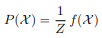
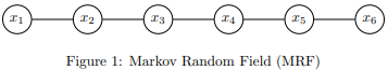
2. Figure 1 shows a Markov Network (MN) encoding the joint distribution

of random variables X = {x1, x2, x3, x4, x5, x6} that each take binary values xj ∈ {−1, +1} for j = 1, · · · , 6. The clique potentials are

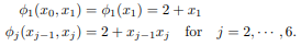
For notational convenience we define the deterministic dummy (“fake”) variable x0 ≡ 1 and write

φj (xj−1, xj ) = 2 + xj−1xj for j = 1, · · · , 6

Note that Figure 1 only shows the true random variables, excluding the dummy variable x0. However, no harm ensues if one rewrites the graph to include the deterministic variable x0.

(a) Write P(X ) in terms of the clique potentials and compute the actual numerical values of the normalization factor Z and P(x1 = +1) and P(x1 = −1) in a numerically efficient manner.

(b) Now suppose that we are able to directly probe the value of node two (and only node two) using a device that provides us with a single scalar measurement y that can take binary values y ∈ {−1, 1}. Given x2, we take y to be independent of all other nodes and we assume that the relationship between the values of x2 and y is captured by an observation potential function

φobs(y, x2) = 4yx2 = 22yx2 .

Suppose that a noisy measurement of x2 is taken resulting in the data value y = −1. Compute the numerical values of P(x1 = +1|y = −1) and P(x1 = −1|y = −1).